Multi-Level Modeling (MLM)

Ekarin E. Pongpipat

Review

If you have any questions, please just stop me. I prefer answering questions as they come up.

Before I go over multi-level modeling, I want to review some information that I think is helpful in understanding it.

Assumptions

The first thing to know about all linear models is that error is assumed to be normal and independent or random

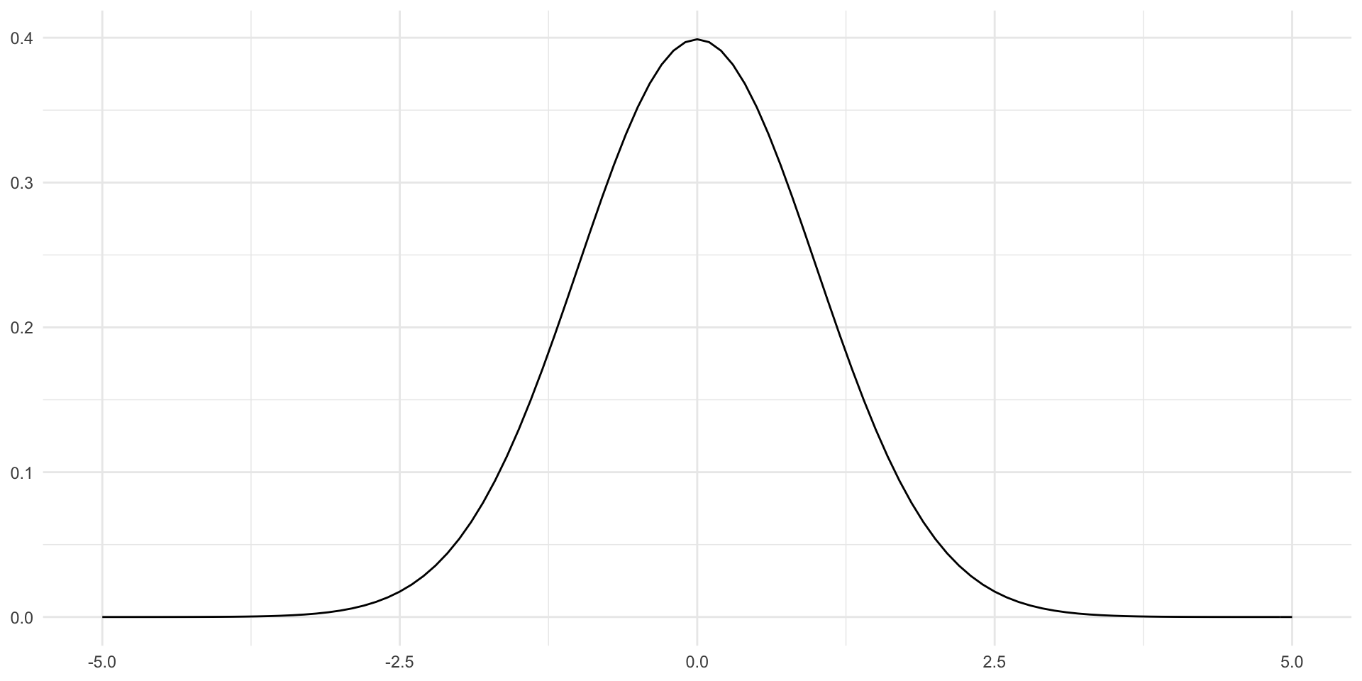
• Error is normal
• Error is independent (random)

Data

So, let’s take a look at how we properly ensure error is independent with two time points. Let’s say that we are interested in the effect of aging – using wave – on digit span (sequence)?

• Two time points per person
• Is there an effect of aging (using wave) on digit span (sequence)?

sub	ses	wave	ds_s
1002	1	-0.5	15
1002	2	0.5	16
1003	1	-0.5	8
1003	2	0.5	12
1005	1	-0.5	12
1005	2	0.5	15

t-test

If we were to properly perform the t-test, we would want to run a dependent samples t-test. The dependent samples t-test takes the difference between the two waves and examines if it is different than 0.

Accounting for subject

(dependent samples t-test)

\[ DS_{S_{W2_i}} - DS_{S_{W1_i}} = \beta_0 + \epsilon_i \]

# A tibble: 1 × 5
  term        estimate std.error statistic p.value
  <chr>          <dbl>     <dbl>     <dbl>   <dbl>
1 (Intercept)    0.182     0.184     0.988   0.325

Incorrectly ignoring subject

(independent samples t-test)

\[ DS_{S_{t_i}} = \beta_0 + \beta_1*Wave_{t_i} + \epsilon_i \]

# A tibble: 2 × 5
  term        estimate std.error statistic   p.value
  <chr>          <dbl>     <dbl>     <dbl>     <dbl>
1 (Intercept)    9.23      0.147    62.9   3.36e-151
2 wave           0.182     0.293     0.620 5.36e-  1

• Same estimate
• Error is wrong in the independent samples t-test (subsequently, t-statistic and p-value)
  • Error is not independent since measures within the same subjects are correlated

Beyond repeated-measures

• What happens if you have more than two time points?
  • Repeated Measures GLM (ANOVA/Regression) and MLM
• However, MLM also allows for missing data points and accounts for multiple sources of error

Definitions

• Multi-Level Modeling (MLM)

• Also known as:

  • Hierarchical Linear Modeling (HLM)
    • Not to be confused with Hierarchical Regression
  • Linear Mixed Effects (LME)
  • Mixed Effects Modeling

Definitions

• Variables can vary within and vary between levels/clusters
• Dependent variables must vary both within and between levels
• Independent variables can vary both within and between levels or only between levels
  • IVs that vary within and between levels are called random
  • IVs that vary only between the highest level are called fixed

Our Longitudinal Data

Example #1: 2 Levels

Multiple cognitive measures or MRI data over time for each individual

• Level 1: Subject-Level
  • Multiple measures across time
• Level 2: Group-Level
  • Multiple subjects

Example #2: 3 levels levels

Multiple related data points within an individual’s wave collected over multiple waves

• Level 1: Within wave
  • Multiple related data points within a wave/time (e.g., accuracies across n-back load)
• Level 2: Within subject (between waves/times)
  • Multiple measures over time
• Level 3: Between subjects
  • Multiple subjects

Error

Multiple Sources of Error

• General linear models (e.g., regression, ANOVA, etc.) only accounts for a single source of model error

\[ DV_i = \beta_0 + \beta_1 * X_i + \epsilon \]

• MLM allows us to account for variability/error within and between different levels

• Level 1: Within-Subject

\[ DV_{t_i} = \beta_{0_i} + \beta_{1_i} * Time_{t_i} + r_{t_i} \]

• Level 2: Between-Subjects

\[ \beta_{0_i} = \gamma_{00} + \gamma_{01} * Age_{W1_i} + \mu_{0_i} \]

\[ \beta_{1_i} = \gamma_{10} + \gamma_{11} * Age_{W1_i} + \mu_{1_i} \]

Error

Level 1

\[ r_{t_i} = N(0, \sigma^2) \]

Level 2

\[ \mu_{t_i} = N(0, \tau_{t_i}) \]

Level 2 Expanded:

\[ \begin{bmatrix} \mu_{0_i}\\ \mu_{1_i} \end{bmatrix} = N \begin{pmatrix} 0, \tau_{00}^2\ \ \tau_{01}\\ 0, \tau_{01}\ \ \tau_{10}^2 \end{pmatrix} \]

Errors within a subject are normal and variance-covariance of errors between subjects are also normal

Steps

1. Define model

2. Data processing

3. Run model

4. Review model

5. Visualize model

Getting Started

Packages

library(dplyr)          # data wrangling
library(lmerTest)       # to run lme
library(interactions)   # to plot interactions

Our Example Data

sub	ses	age	cesd	ds_s	age_w1	sex	time	female
1002	1	57	2	15	57	M	0	0
1002	2	62	4	16	57	M	5	0
1002	3	66	0	16	57	M	9	0
1003	1	37	11	8	37	F	0	1
1003	2	42	11	12	37	F	5	1
1004	1	30	7	8	30	F	0	1

Example #1

Example #1

Time Points: 2

variable	effect	varies
intercept	random	within subject
time	fixed	between subjects

Define

Level 1

\[ DS\_S = \beta_{0_i} + r_{i_t} \]

Level 2

\[ \beta_{0_i} = \gamma_{00} + \gamma_{01} * Time_i + \mu_{0_i} \]

Full Model

\[ \begin{align} DS\_S_{t_i} & = (\gamma_{00} + \gamma_{01} * Time_i + \mu_{0_i}) + r_{t_i} \\ & = \gamma_{00} + \gamma_{01} * Time_i + \mu_{0_i} + r_{t_i} \end{align} \]

Mean-Center

df_long_2ses <- df_long_2ses %>%
  mutate(time_mc = scale(time, scale = F))

sub	ses	age	cesd	ds_s	age_w1	sex	time	female	time_mc
1002	1	57	2	15	57	M	0	0	-1.520833
1002	2	62	4	16	57	M	5	0	3.479167
1003	1	37	11	8	37	F	0	1	-1.520833
1003	2	42	11	12	37	F	5	1	3.479167
1004	1	30	7	8	30	F	0	1	-1.520833
1005	1	21	6	12	21	F	0	1	-1.520833

typically, mean-center if there is an interaction (unless if your variable and estimate are meaningful at 0).

Run

General format:

model_fit <- lmer(dv ~ full_model + (level_1_model | id), data)

Code:

model_fit <- lmer(ds_s ~ time_mc + (1 | sub), df_long_2ses)

Review

summary(model_fit)

Linear mixed model fit by REML. t-tests use Satterthwaite's method [
lmerModLmerTest]
Formula: ds_s ~ time_mc + (1 | sub)
   Data: df_long_2ses

REML criterion at convergence: 1443.9

Scaled residuals: 
    Min      1Q  Median      3Q     Max 
-4.1345 -0.4349 -0.0471  0.3339  2.9746 

Random effects:
 Groups   Name        Variance Std.Dev.
 sub      (Intercept) 2.936    1.713   
 Residual             2.022    1.422   
Number of obs: 336, groups:  sub, 215

Fixed effects:
             Estimate Std. Error        df t value            Pr(>|t|)    
(Intercept)   9.22001    0.14225 214.33908  64.818 <0.0000000000000002 ***
time_mc       0.03664    0.04077 150.21252   0.899                0.37    
---
Signif. codes:  0 '***' 0.001 '**' 0.01 '*' 0.05 '.' 0.1 ' ' 1

Correlation of Fixed Effects:
        (Intr)
time_mc 0.062 

Review

b <- coef(model_fit)[[1]]
head(b)

     (Intercept)    time_mc
1002   13.864461 0.03664226
1003    9.773489 0.03664226
1004    8.530614 0.03664226
1005   12.390462 0.03664226
1006   10.145395 0.03664226
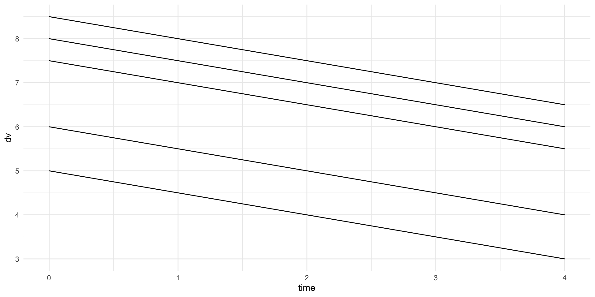
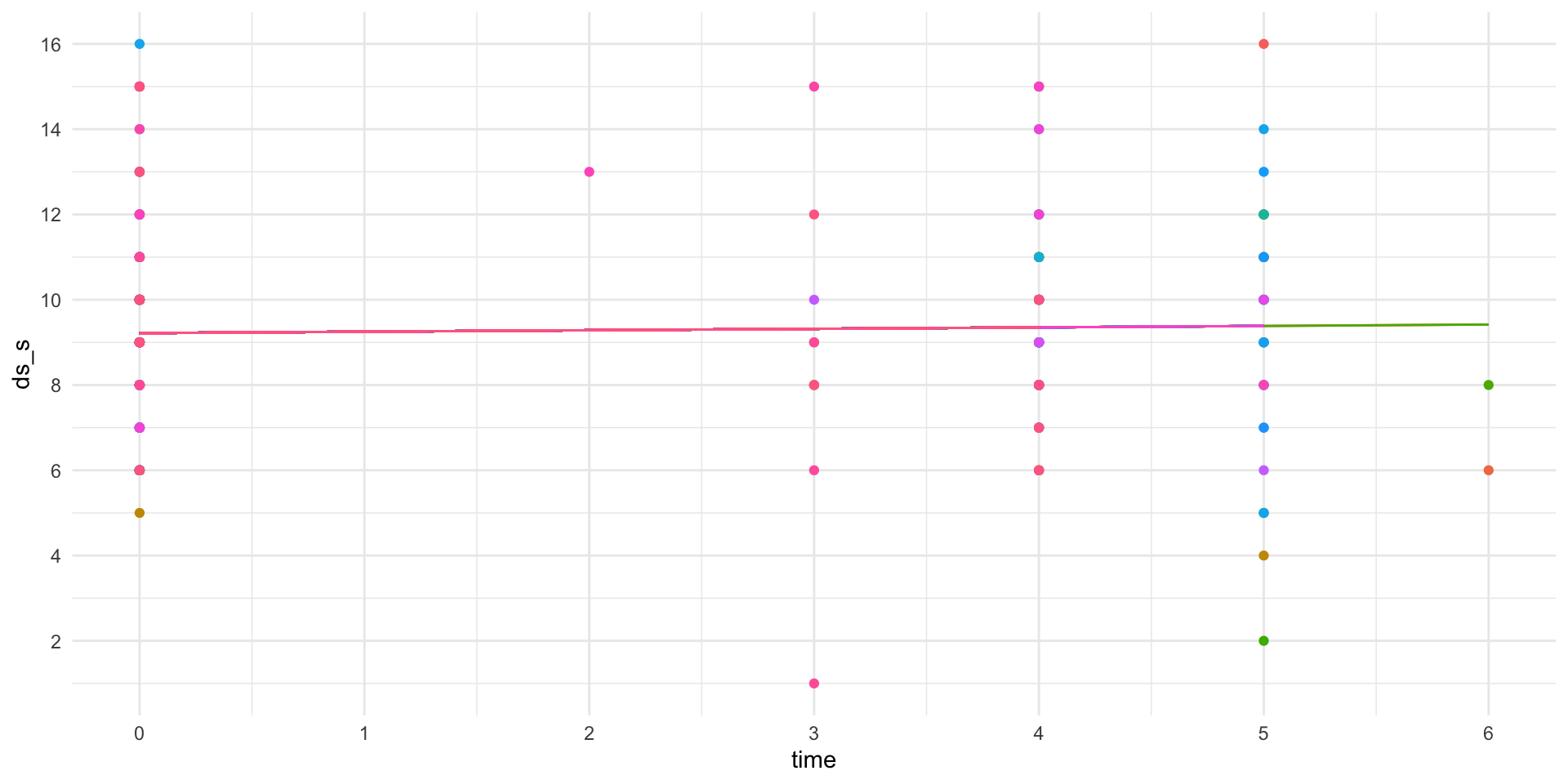
1007    8.644142 0.03664226

mean(b[, '(Intercept)'])

[1] 9.220007

Visualize

The slope is the same, but the intercept is different (random/varies within subject)

Example #2

Example #2

Time Points: 2

variable	effect	varies
intercept	fixed	between subjects
time	random	varies subject

Define

Level 1

\[ DS\_S_{t_i} = \beta_{0_i} + \beta_{1_i} * Time_{t_i} + r_{t_i} \]

where \(\beta_0 = 0\)

Level 2

\[ \beta_{0_i} = \gamma_{00} + \mu_{0_i} \]

\[ \beta_{1_i} = \gamma_{10} + \mu_{1_i} \]

Full Model

\[ \begin{align} DS\_S_{t_i} & = (\gamma_{00} + \mu_{0_i}) + (\gamma_{10} + \mu_{1_i}) + r_{t_i} \\ & = \gamma_{00} + \gamma_{10} + r_{i_t} + \mu_{0_i} + \mu_{1_i} \end{align} \]

Run

model_fit <- lmer(ds_s ~ time_mc + (0 + time_mc | sub), df_long_2ses)

Note: R automatically includes to the intercept and we have to explicitly state 0 to have a fixed intercept

Review

summary(model_fit)

Linear mixed model fit by REML. t-tests use Satterthwaite's method [
lmerModLmerTest]
Formula: ds_s ~ time_mc + (0 + time_mc | sub)
   Data: df_long_2ses

REML criterion at convergence: 1498.8

Scaled residuals: 
    Min      1Q  Median      3Q     Max 
-3.6953 -0.5813 -0.0743  0.3727  3.0547 

Random effects:
 Groups   Name    Variance Std.Dev.
 sub      time_mc 0.000    0.000   
 Residual         5.005    2.237   
Number of obs: 336, groups:  sub, 215

Fixed effects:
             Estimate Std. Error        df t value            Pr(>|t|)    
(Intercept)   9.21726    0.12204 334.00000  75.524 <0.0000000000000002 ***
time_mc       0.03351    0.05912 334.00000   0.567               0.571    
---
Signif. codes:  0 '***' 0.001 '**' 0.01 '*' 0.05 '.' 0.1 ' ' 1

Correlation of Fixed Effects:
        (Intr)
time_mc 0.000 
optimizer (nloptwrap) convergence code: 0 (OK)
boundary (singular) fit: see ?isSingular

Review

b <- coef(model_fit)[[1]]
head(b)

     (Intercept)    time_mc
1002    9.217262 0.03350842
1003    9.217262 0.03350842
1004    9.217262 0.03350842
1005    9.217262 0.03350842
1006    9.217262 0.03350842
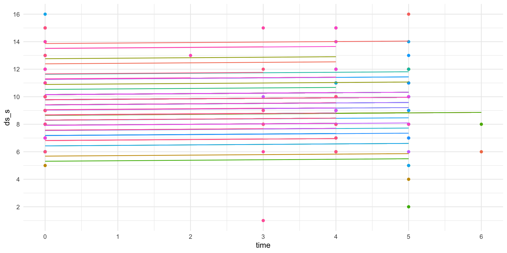
1007    9.217262 0.03350842

Visualize

Example #3

Example #3

Time Points: 2

variable	effect	varies
intercept	fixed	between subject
time	random	within subject
age_w1	fixed	between subjects

Define

Level 1

\[ DS\_S_{i_t} = \beta_{0_i} + \beta_{1_i} * Time_{i_t} + r_{i_t} \]

where \(\beta_0 = 0\)

Level 2

\[ \beta_{0_i} = \gamma_{00} + \gamma_{01} * Age_{W1_i} + \mu_{0_i} \]

\[ \beta_{1_i} = \gamma_{10} + \gamma_{11} * Age_{W1_i} + \mu_{1_i} \]

Full Model

\[ \begin{align} \begin{split} DS\_S_{i_t} &= (\gamma_{00} + \gamma_{01} * Age_{W1_i} + \mu_{0_i}) + (\gamma_{10} + \gamma_{11} * Age_{W1_i} + \mu_{1_i})*Time_{t_i} + r_{i_t} \\ &= \gamma_{00} + \gamma_{01} * Age_{W1_i} + \gamma_{10}*Time_{t_i} + \gamma_{11} * Age_{W1_i} *Time_{t_i} \\ &\qquad + r_{i_t} + \mu_{0_i} + \mu_{1_i} \end{split} \end{align} \]

Mean-Center

m_age_w1 <- mean(subset(df_long_2ses, ses == 1)$age)
df_long_2ses <- df_long_2ses %>%
  mutate(age_w1_mc = age_w1 - m_age_w1)

sub	ses	age	cesd	ds_s	age_w1	sex	time	female	time_mc	age_w1_mc
1002	1	57	2	15	57	M	0	0	-1.520833	3.204651
1002	2	62	4	16	57	M	5	0	3.479167	3.204651
1003	1	37	11	8	37	F	0	1	-1.520833	-16.795349
1003	2	42	11	12	37	F	5	1	3.479167	-16.795349
1004	1	30	7	8	30	F	0	1	-1.520833	-23.795349
1005	1	21	6	12	21	F	0	1	-1.520833	-32.795349

Run

model_fit <- lmer(ds_s ~ time_mc * age_w1_mc + (0 + time_mc | sub), df_long_2ses)

Note: R automatically includes to the intercept and we have to explicitly state 0 to have a fixed intercept

Review

summary(model_fit)

Linear mixed model fit by REML. t-tests use Satterthwaite's method [
lmerModLmerTest]
Formula: ds_s ~ time_mc * age_w1_mc + (0 + time_mc | sub)
   Data: df_long_2ses

REML criterion at convergence: 1458.5

Scaled residuals: 
    Min      1Q  Median      3Q     Max 
-3.3755 -0.7105 -0.0439  0.5528  3.6532 

Random effects:
 Groups   Name    Variance Std.Dev.
 sub      time_mc 0.000    0.000   
 Residual         4.226    2.056   
Number of obs: 336, groups:  sub, 215

Fixed effects:
                    Estimate Std. Error         df t value             Pr(>|t|)
(Intercept)         9.249069   0.112266 332.000000  82.385 < 0.0000000000000002
time_mc             0.049013   0.054381 332.000000   0.901                0.368
age_w1_mc          -0.048459   0.006127 332.000000  -7.910   0.0000000000000387
time_mc:age_w1_mc  -0.004309   0.003022 332.000000  -1.426                0.155
                     
(Intercept)       ***
time_mc              
age_w1_mc         ***
time_mc:age_w1_mc    
---
Signif. codes:  0 '***' 0.001 '**' 0.01 '*' 0.05 '.' 0.1 ' ' 1

Correlation of Fixed Effects:
            (Intr) tim_mc ag_w1_
time_mc      0.002              
age_w1_mc   -0.032 -0.032       
tm_mc:g_w1_ -0.033 -0.031  0.058
optimizer (nloptwrap) convergence code: 0 (OK)
boundary (singular) fit: see ?isSingular

Review

b <- coef(model_fit)[[1]]
head(b)

     (Intercept)   time_mc  age_w1_mc time_mc:age_w1_mc
1002    9.249069 0.0490125 -0.0484594      -0.004309302
1003    9.249069 0.0490125 -0.0484594      -0.004309302
1004    9.249069 0.0490125 -0.0484594      -0.004309302
1005    9.249069 0.0490125 -0.0484594      -0.004309302
1006    9.249069 0.0490125 -0.0484594      -0.004309302
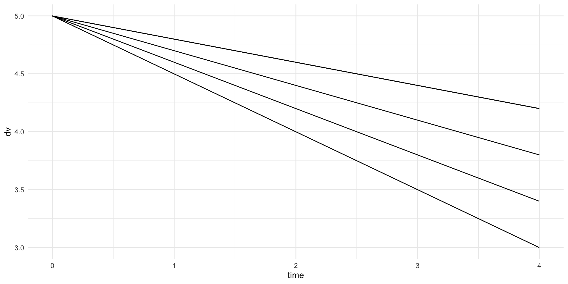
1007    9.249069 0.0490125 -0.0484594      -0.004309302

Visualize

# re-run without centering for interactions plot only
model_fit_fig <- lmer(ds_s ~ time * age_w1 + (0 + time | sub), df_long_2ses) 
interact_plot(model_fit_fig, pred = time, modx = age_w1, plot.points = TRUE) +
  scale_x_continuous(breaks = seq(0, 20, 1))

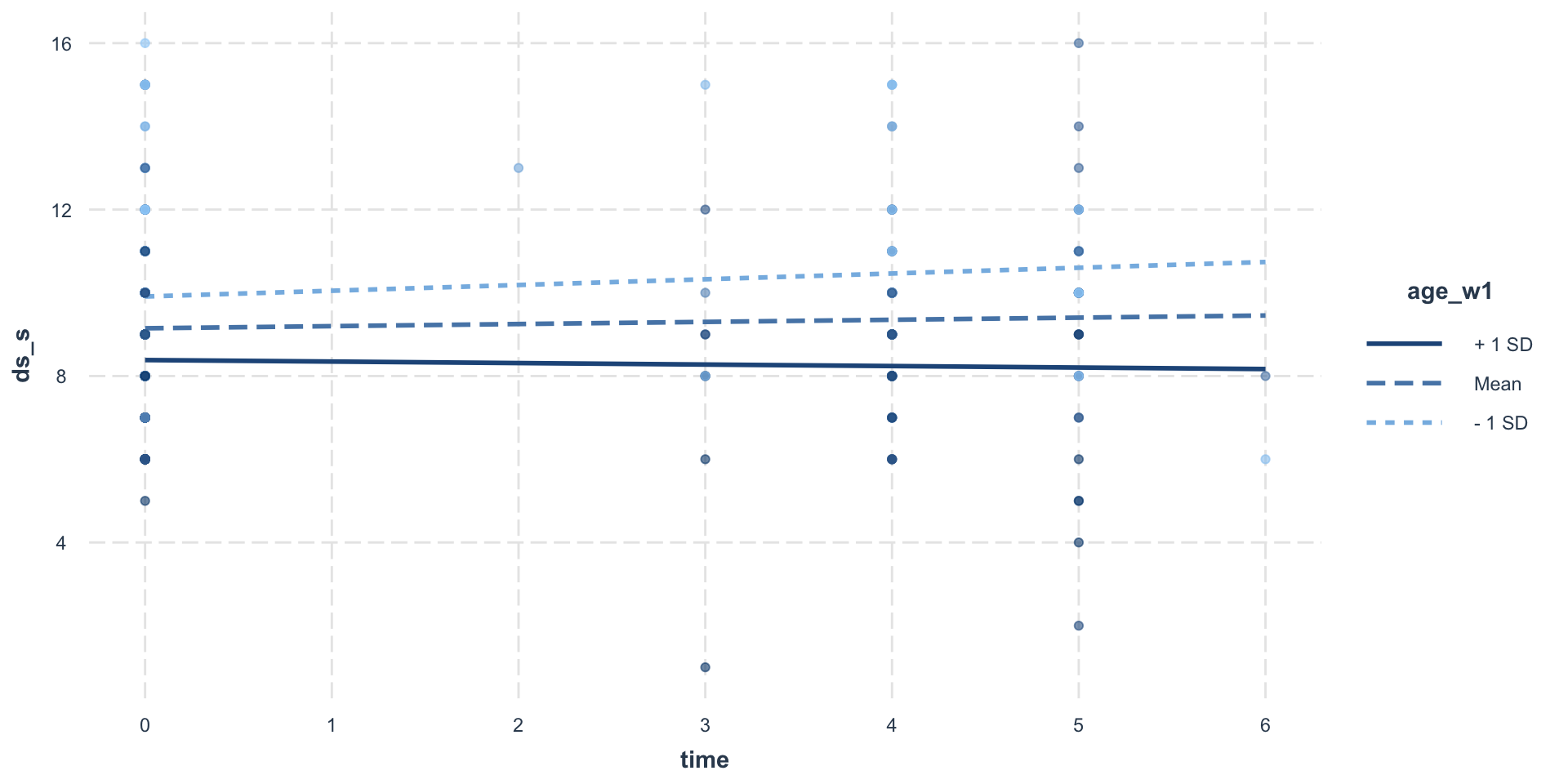
Visualize

Example #4

Example #4

Time Points: 3

variable	effect	varies
intercept	random	within subject
time	random	within subject
age_w1	fixed	between subjects
sex	fixed	between subjects

Define

Level 1

\[ DS\_S_{t_i} = \beta_{0_i} + \beta_{1_i} * Time_{t_i} + r_{t_i} \]

Level 2

\[ \beta_{0_i} = \gamma_{00} + \gamma_{01} * Age_{W1_i} + \gamma_{02} * Sex_i + \gamma_{03} * Age_{W1_i} * Sex_i + \mu_{0_i} \]

\[ \beta_{1_i} = \gamma_{10} + \gamma_{11} * Age_{W1_i} + \gamma_{12} * Sex_i + \gamma_{13} * Age_{W1_i} * Sex_i + \mu_{1_i} \]

Full Model

\[ \begin{split} DS\_S_{i_t} &= (\gamma_{00} + \gamma_{01} * Age_{W1_i} + \gamma_{02} * Sex_i + \gamma_{03} * Age_{W1_i} * Sex_i + \mu_{0_i}) \\ &\qquad + (\gamma_{10} + \gamma_{11} * Age_{W1_i} + \gamma_{12} * Sex_i + \gamma_{13} * Age_{W1_i} * Sex_i + \mu_{1_i}) * Time_{i_t} \\ &\qquad + r_{i_t} \end{split} \]

Define

Full Model

\[ \begin{align} \begin{split} DS\_S_{i_t} & = (\gamma_{00} + \gamma_{01} * Age_{W1_i} + \gamma_{02} * Sex_i + \gamma_{03} * Age_{W1_i} * Sex_i + \mu_{0_i}) \\ &\qquad + (\gamma_{10} + \gamma_{11} * Age_{W1_i} + \gamma_{12} * Sex_i + \gamma_{13} * Age_{W1_i} * Sex_i + \mu_{1_i}) * Time_{i_t} \\ &\qquad + r_{i_t} \\ & = \gamma_{00} + \gamma_{01} * Age_{W1_i} + \gamma_{02} * Sex_i + \gamma_{03} * Age_{W1_i} * Sex_i \\ &\qquad + \gamma_{10} * Time_{i_t} + \gamma_{11} * Age_{W1_i} * Time_{i_t} + \gamma_{12} * Sex_i * Time_{i_t} \\ &\qquad + \gamma_{13} * Age_{W1_i} * Sex_i * Time_{i_t} \\ &\qquad + r_{i_t} + \mu_{0_i} + \mu_{1_i} \end{split} \end{align} \]

Run

df_long <- df_long %>%
  mutate(age_w1_mc = age_w1 - m_age_w1,
         time_mc = scale(time, scale = F),
         female_c = ifelse(sex == 'F', 0.5, -0.5))
head(df_long)

   sub ses age cesd ds_s age_w1 sex time female  age_w1_mc   time_mc female_c
1 1002   1  57    2   15     57   M    0      0   3.204651 -2.478589     -0.5
2 1002   2  62    4   16     57   M    5      0   3.204651  2.521411     -0.5
3 1002   3  66    0   16     57   M    9      0   3.204651  6.521411     -0.5
4 1003   1  37   11    8     37   F    0      1 -16.795349 -2.478589      0.5
5 1003   2  42   11   12     37   F    5      1 -16.795349  2.521411      0.5
6 1004   1  30    7    8     30   F    0      1 -23.795349 -2.478589      0.5

model_fit <- lmer(ds_s ~ time_mc * age_w1_mc * female_c + (1 + time_mc | sub), df_long)

Review

summary(model_fit)

Linear mixed model fit by REML. t-tests use Satterthwaite's method [
lmerModLmerTest]
Formula: ds_s ~ time_mc * age_w1_mc * female_c + (1 + time_mc | sub)
   Data: df_long

REML criterion at convergence: 1309.7

Scaled residuals: 
    Min      1Q  Median      3Q     Max 
-3.8063 -0.5107 -0.0179  0.4543  2.9256 

Random effects:
 Groups   Name        Variance Std.Dev. Corr
 sub      (Intercept) 2.34389  1.531        
          time_mc     0.02657  0.163    0.03
 Residual             1.86809  1.367        
Number of obs: 308, groups:  sub, 126

Fixed effects:
                             Estimate Std. Error         df t value
(Intercept)                  9.287386   0.165912 120.240758  55.978
time_mc                     -0.001836   0.032633  93.289540  -0.056
age_w1_mc                   -0.045366   0.009629 121.590599  -4.712
female_c                    -0.064794   0.331825 120.240758  -0.195
time_mc:age_w1_mc           -0.002910   0.001913  95.118994  -1.521
time_mc:female_c             0.021861   0.065266  93.289540   0.335
age_w1_mc:female_c          -0.016199   0.019257 121.590599  -0.841
time_mc:age_w1_mc:female_c  -0.001364   0.003827  95.118994  -0.356
                                       Pr(>|t|)    
(Intercept)                < 0.0000000000000002 ***
time_mc                                   0.955    
age_w1_mc                             0.0000066 ***
female_c                                  0.846    
time_mc:age_w1_mc                         0.132    
time_mc:female_c                          0.738    
age_w1_mc:female_c                        0.402    
time_mc:age_w1_mc:female_c                0.722    
---
Signif. codes:  0 '***' 0.001 '**' 0.01 '*' 0.05 '.' 0.1 ' ' 1

Correlation of Fixed Effects:
            (Intr) tim_mc ag_w1_ feml_c tm_:_1_ tm_m:_ a_1_:_
time_mc     -0.067                                           
age_w1_mc    0.026 -0.020                                    
female_c    -0.247  0.031 -0.147                             
tm_mc:g_w1_ -0.020 -0.026 -0.059  0.021                      
tm_mc:fml_c  0.031 -0.183  0.021 -0.067 -0.120               
ag_w1_mc:f_ -0.147  0.021 -0.344  0.026  0.044  -0.020       
tm_mc:_1_:_  0.021 -0.120  0.044 -0.020 -0.237  -0.026 -0.059

Review

b <- coef(model_fit)[[1]]
head(b)

     (Intercept)     time_mc  age_w1_mc    female_c time_mc:age_w1_mc
1002   14.201984  0.13504522 -0.0453662 -0.06479377      -0.002910267
1003    9.185039  0.10800557 -0.0453662 -0.06479377      -0.002910267
1005   11.137925  0.05868963 -0.0453662 -0.06479377      -0.002910267
1006   10.111018  0.02322896 -0.0453662 -0.06479377      -0.002910267
1007    7.898931 -0.20021379 -0.0453662 -0.06479377      -0.002910267
1010    9.308339 -0.05749068 -0.0453662 -0.06479377      -0.002910267
     time_mc:female_c age_w1_mc:female_c time_mc:age_w1_mc:female_c
1002        0.0218611        -0.01619893               -0.001363629
1003        0.0218611        -0.01619893               -0.001363629
1005        0.0218611        -0.01619893               -0.001363629
1006        0.0218611        -0.01619893               -0.001363629
1007        0.0218611        -0.01619893               -0.001363629
1010        0.0218611        -0.01619893               -0.001363629

Visualize

model_fit_fig <- lmer(ds_s ~ time * age_w1 * sex + (1 + time_mc | sub), df_long)
interact_plot(model_fit_fig, pred = time, modx = age_w1, mod2 = sex, plot.points = TRUE) +
  scale_x_continuous(breaks = seq(0, 20, 1))

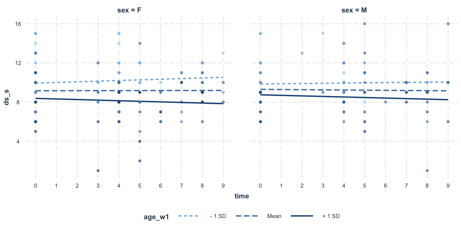
Visualize

Missingness

	type	abbreviation	definition	note
1	Missing Completely at Random	MCAR	Truly random process	Ideal
2	Missing at Random	MAR	Not completely missing at random and missingness is a measured/predictable process	OK
3	Missing Not at Random	MNAR	Not missing at random, and unmeasured/unpredictable	Bad

Pattern Mixture Modeling

Pattern Mixture Modelling

“Extension” of MLM by including a missingness variable

• Create contrast variables of missingness pattern
  • Examples:
    • dummy-coded variable of complete observations
    • dummy-coded variable of missing last wave/session
    • number of waves/sessions
    • all missingness patterns
• Control for main effect missingness or determine if there is an interaction of variables with missingness

Example

Let’s incldue all patterns as control/nuisance variables

In our case, we have 4 patterns of missing:

1. CCC - completed all waves
2. CCM - completed first two waves and missing last wave
3. CMC - completed first and third wave and missing second wave
4. CMM - completed first wave and missing last two waves

Create variables

• Create missing data patterns

df_missing <- df_wide %>%
  filter(sub %in% df_long$sub) %>%
  mutate(missing = case_when(
    !is.na(time_w1) & !is.na(time_w2) & !is.na(time_w3) ~ 0,
    !is.na(time_w1) & !is.na(time_w2) &  is.na(time_w3) ~ 1,
    !is.na(time_w1) &  is.na(time_w2) & !is.na(time_w3) ~ 2,
    !is.na(time_w1) &  is.na(time_w2) &  is.na(time_w3) ~ 3
  )) %>%
  select(sub, contains('missing'))
head(df_missing)

   sub missing
1 1002       0
2 1003       1
3 1005       1
4 1006       0
5 1007       1
6 1010       0

report::report(as.factor(df_missing$missing))

x: 3 levels, namely 0 (n = 56, 44.44%), 1 (n = 65, 51.59%) and 2 (n = 5, 3.97%)

# dummy code
df_missing <- df_missing %>%
  dummy_cols(select_columns = 'missing')
head(df_missing)

   sub missing missing_0 missing_1 missing_2
1 1002       0         1         0         0
2 1003       1         0         1         0
3 1005       1         0         1         0
4 1006       0         1         0         0
5 1007       1         0         1         0
6 1010       0         1         0         0

Run

Combine

# merge back to data
df_long <- df_long %>%
  left_join(df_missing, by = 'sub') #%>%
  # filter(n_ses >= 2)

Run

model_fit <- lmer(ds_s ~ time_mc * age_w1_mc * female_c + missing_1 + missing_2 + (1 + time_mc | sub), df_long)

Review

summary(model_fit)

Linear mixed model fit by REML. t-tests use Satterthwaite's method [
lmerModLmerTest]
Formula: ds_s ~ time_mc * age_w1_mc * female_c + missing_1 + missing_2 +  
    (1 + time_mc | sub)
   Data: df_long

REML criterion at convergence: 1306

Scaled residuals: 
    Min      1Q  Median      3Q     Max 
-3.7570 -0.4715 -0.0044  0.4458  2.9634 

Random effects:
 Groups   Name        Variance Std.Dev. Corr
 sub      (Intercept) 2.33027  1.5265       
          time_mc     0.02628  0.1621   0.02
 Residual             1.87168  1.3681       
Number of obs: 308, groups:  sub, 126

Fixed effects:
                             Estimate Std. Error         df t value
(Intercept)                  9.555692   0.238187 112.038680  40.118
time_mc                     -0.006995   0.032840  95.107419  -0.213
age_w1_mc                   -0.048554   0.009849 119.464405  -4.930
female_c                     0.010915   0.334868 118.231360   0.033
missing_1                   -0.493858   0.330820 120.324457  -1.493
missing_2                   -0.772077   0.865639 123.500338  -0.892
time_mc:age_w1_mc           -0.002915   0.001912  95.337461  -1.525
time_mc:female_c             0.022290   0.065194  93.391498   0.342
age_w1_mc:female_c          -0.014557   0.019252 119.676547  -0.756
time_mc:age_w1_mc:female_c  -0.001443   0.003823  95.166854  -0.377
                                       Pr(>|t|)    
(Intercept)                < 0.0000000000000002 ***
time_mc                                   0.832    
age_w1_mc                            0.00000268 ***
female_c                                  0.974    
missing_1                                 0.138    
missing_2                                 0.374    
time_mc:age_w1_mc                         0.131    
time_mc:female_c                          0.733    
age_w1_mc:female_c                        0.451    
time_mc:age_w1_mc:female_c                0.707    
---
Signif. codes:  0 '***' 0.001 '**' 0.01 '*' 0.05 '.' 0.1 ' ' 1

Correlation of Fixed Effects:
            (Intr) tim_mc ag_w1_ feml_c mssn_1 mssn_2 tm_:_1_ tm_m:_ a_1_:_
time_mc     -0.132                                                         
age_w1_mc   -0.115 -0.005                                                  
female_c    -0.077  0.021 -0.174                                           
missing_1   -0.709  0.118  0.162 -0.115                                    
missing_2   -0.275 -0.003  0.179 -0.116  0.224                             
tm_mc:g_w1_ -0.017 -0.027 -0.061  0.019 -0.001  0.027                      
tm_mc:fml_c  0.023 -0.181  0.020 -0.073  0.002 -0.011 -0.121               
ag_w1_mc:f_ -0.068  0.018 -0.348  0.034 -0.042 -0.047  0.046  -0.020       
tm_mc:_1_:_  0.003 -0.117  0.048 -0.022  0.017  0.001 -0.237  -0.026 -0.067
optimizer (nloptwrap) convergence code: 0 (OK)
Model failed to converge with max|grad| = 0.0025705 (tol = 0.002, component 1)

Warnings: isSingular

boundary (singular) fit: see ?isSingular

• Possibly, at least one of the variances within or correlations between the random effects is either 0 or ±1.
  • try setting the parameter of the covariance of the residuals (\(tau_{01}\)) to not be estimated (1 + time || sub)

References

• https://rpsychologist.com/r-guide-longitudinal-lme-lmer
• https://www.learn-mlms.com/index.html
• https://jeanettemumford.org/MixedModelSeries/